COMMANDS FOR BUILDING GRAPHIC PRIMITIVES
Laboratory work.
Ways to set point coordinates and select objects.
There are four ways to specify the coordinates of a point.
1. One way is to enter absolute Cartesian coordinates (type X, Y at the command line).

2. Assignment of the coordinate of the point relative to the previous one in increment of abscissa and ordinate @ X, Y. The @ sign means entering relative coordinates.

3. Entering the coordinate of a point using polar coordinates implies setting a point relative to the previous one by the distance between them and the angle of rotation. The entry form on the command line will look like:
@L <.

4. The last way to set the coordinates of a point is to specify the coordinates directly by the “mouse” on the screen itself.
Laboratory work
Building graphic primitives
Access to graphic primitives in the ribbon interface is implemented using the Home tab in the workspace Drawing and annotations (Fig. 4.1)

Fig. 4.1 Access to graphical primitives in the ribbon interface
In addition, to build graphic primitives, you can select the special Drawing toolbar or the drop-down menu item of the same name (Fig. 4.2).

Fig. 4.2 Drop-down menu item. Painting
The most common graphic primitives are as a segment, line, circle, arc, rectangle, point, ellipse, etc. Their construction is elementary, you just need to follow the dialogue on the command line.
For example, a circle can be displayed in five ways. Among them - the construction of a circle at two points, which determines the coordinates of the diameter of the circle; plotting a circle along two tangents and a radius, etc.
Laboratory work.
AutoCAD Compound Objects
AutoCAD composite objects are designed to facilitate and accelerate the construction of drawings, to obtain high quality graphic objects. So, the use of Polyline - a combination of linear and arc segments, perceived as a whole - greatly facilitates the work with objects created on their basis. One of the options for quickly creating a polyline consisting of only arc segments is the Cloud command Revcloud, which allows you to create closed areas for entering various annotations on the drawing. With the help of Multiline - a set of parallel lines of various types and colors - it is easy to build a bundle of parallel pipes or a road map. Regions and Boundary allow you to create complex shapes based on existing relatively simple objects. Hatching allows you to quickly and accurately perform hatching of objects of various shapes.
Polyline 
Polyline is a continuous sequence of rectilinear segments and arcs that are considered as a whole system. AutoCAD uses two types of polylines - two-dimensional and three-dimensional.
The main differences between a polyline and simple segments and arcs in contact with end points:
- the polyline is processed as a single object;
- each individual segment of a polyline can have any width, including a variable;
- the sequence of segments and arcs can form a closed shape in the form of a rectangle or polygon;
- commands for editing Chamfer and Fillet objects are applied simultaneously for all vertices of a polyline;
- polylines can be smooth and turned into a spline;
- the vertices of the polyline can be edited by adding or removing them.
In addition, AutoCAD allows you to calculate the area covered by the polyline and its perimeter.
Hatching
Hatching can be done using one of the standard hatch patterns supplied with AutoCAD, a sample created by the user and saved in a special file for future use, or a set of lines located at any angle set during the hatch process (Fig. 4.3).
Standard and user-defined hatch patterns in the hatching process can be scaled and the angle of inclination of lines in them can be changed. When performing hatching with separate lines, it is possible to change the angle of inclination of the lines, the distance between the lines, and also arrange them crosswise.
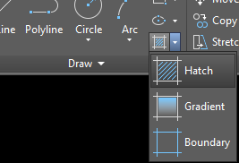
Figure 4.3 Accessing hatching using a tape interface
For engineering drawings, the most acceptable shading is called ANSI 31, the reference to which is specified in the sample window (Fig. 4.4)

Fig. 4.4 Hatch and Gradient Dialog Box (collapsed version)
Hatching (dashed block) can be divided into its individual elements, segments. Such an operation can be performed using the Explode edit command.
Hatching is preferably performed on a separate layer. In this case, its output can be easily controlled by freezing or turning off this layer. The use of various hatching options is possible with the help of tool palettes (see Fig. 3.10).
Gradient fill is a smooth transition of one color to another or a smooth change in tonality for one color. In AutoCAD, you can use either a two-color gradient fill, or a fill consisting of shades of the same color. Unlike hatching, it cannot be dissected. When creating a gradient fill, it is possible to select one of nine types of gradients, change the angle of the location of the fill, and also set the fill with an offset.
Tables in AutoCAD
Tables are a rectangular array of cells that can contain multi-line text, various characters, special field objects, and also blocks. You can put numerical values in the table and perform various mathematical calculations on them.
The tables are inserted in the ribbon interface from the Annotations tab. The dialog box is reflected in (Fig. 4.5)

Fig. 4.5 Dialog box the Insert table
The inset table in the figure can be accomplished in one of two ways, which is selected in the Method area of the window insert the Insert table.
1. By specifying the insertion point mode Insertion point Sресify.
2. By entering the coordinates of two points, dynamically defining the plot area of a table — mode Specify window.
The first method is used to create a table with a fixed, pre-set number and sizes of rows and columns, the second — when the number and size of rows and columns are specified dynamically in the process of placing the table in the figure.
To insert a table with fixed sizes, you select the checkbox in the Query field, the insertion point, and then in the area of rows and columns to specify the number of columns and rows and width of columns and height of rows. However, note that setting the column Width is set in units of measure adopted in the figure, and setting the row Height by entering the number of lines of text entered in a cell. Therefore, the real height of the rows will depend on the size (height characters) text and fields around him set in the table style.
When you select the second mode of insertion in a zone of Rows and columns dialog box the Insert table displays optional switches that allow you to control the settings that determine how the table is created.
Selecting the checkbox in a particular item specifies a fixed value for the selected parameter, while the corresponding parameter will be determined dynamically. So, if you set the check box for the Number of columns, and set this parameter to 5, then when you insert a table it will create 5 columns, but their width will be determined depending on the region that you specify when you insert a table.
Interesting graphic primitive is a SPLINE
 Spline is the smooth curve, which is based on some set of points.
By default, this smooth curve must pass through all user-defined point. It is mostly used in the drawings to build cliff lines, private cuts (see Fig.4.6).
Click Spline on the toolbar Draw, and then specify the object, namely a polyline that was created with the option Spline command Pedit. Although the appearance of the object may remain the same, its representation in the database of the drawing when this conversion will change.
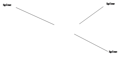

Fig. 4.6. An example of using the Spline command
Consider the options of the command Spline.
Close. Option closes the spline, connecting the last point a continuous curve with the first, according to the given direction of the tangent. It can be specified by choosing some point (while watching the spline changes) or pressing the Enter key. The last case will be set the default tangent direction.
Fit Tolerance. Using this option, you must specify how close to the selected points must be performed spline. The default value of 0, i.e. the spline will pass exactly through the selected points. If the spline is necessary to hold with an error of 0.5 units, then this option should be set to a value of 0.5.
Specify next point(Specify next point). This option is the default. It organizes the input of the next control point of the spline. To complete the process of specifying points, press enter.
Specify the tangent at the start point(Start tangent). After point selection, AutoCAD prompts you to specify tangent direction at the start and end points of the curve. To select the default directions in response to both the prompt and press Enter. Thus, moving the points that define the tangent direction, it is possible to simultaneously monitor the changes of the spline, the resulting displacement.
Laboratory work.
Get help
 There are some very helpful commands of reference information about the objects created. Group reference button operations are shown on the Utilities panel (Fig. 4.7). For these commands, you can also contact by falling of Tools Inquiry.
Almost all these commands request objects (for example, DIST– two points) and display your results in a text window.

Рис.4.7 Utilities panel

Рис. 4.8. Inquiry
EDIT COMMANDS
Laboratory work.
Editing graphic primitives
Ways to select objects
Consider possible ways to select objects.
1. Point - the choice of an object using a point. It is carried out by indicating the coordinates of any point belonging to this object.
2. Sight of the selection of the object. The cursor is automatically replaced by air defense. If an object is selected, it will be displayed on the screen as dots.
For the correct selection of objects, it is necessary to point to the edge of the polyline with a sight, as shown in Fig. 5.1.

Fig. 5.1. Object selection
3. Window. A lot of choices will include those graphic primitives that completely fall into the window


Fig. 5.2. Window selection


 Fig.5.3 Selected objects are highlighted
with hatched line
4. The Wpolygon parameter is similar to the Window parameter, except this time the frame is created in the shape of a regular polygon. AutoCAD selects those objects that are completely located inside this frame.
5. Cut polygon (CPolygon) - similar to the Crossing parameter, except that the frame is created in the form of a regular polygon. AutoCAD selects those objects that are fully or partially located within this frame.
6. One (Single). The user selects only one object, after which AutoCAD will complete the selection process automatically.
After considering the methods of selecting objects, you can proceed to editing commands designed to modify existing primitives and groups of primitives.
To implement editing of graphic primitives, you can select the special editing toolbar (Fig. 5.8) or the drop-down menu item of the same name in the classic AutoCAD workspace.
Editing graphic primitives is also possible in the tape interface using the Main window tab Editing in the workspace Drawing and annotations (Fig. 5.9)

Fig.5.5 address to edit graphic primitives in the ribbon interface
Command ERASE
 Command ERASE allows the user to delete an object or group of objects. The command is very simple and it has almost no options.
The selected object appears as a dotted line. After selecting all objects when you press Enter they will be removed.
Command MOVE
 Command MOVE allows the user to move selected objects from one place to another without changing the orientation of objects.
Shift method: you can enter the shift parameter in the coordinates of the point where the object will be moved, relative to the point used to select an object. The word shift implies the relative nature of the lookup parameter, so the @ symbol when specifying a coordinate is not used. To request a Second point or<to consider the offset of the first point>:press Enter because all the necessary information already entered.
The base point/second point: you can specify a base point anywhere on the drawing, and in response to the query a Second point or<to consider the offset of the first point> would be to determine the distance and the rotation angle or specify a second point. In this case, you can use directly by sight or to enter relative coordinates with the @symbol.
Command STRETCH
 Command STRETCH generally used to stretch groups of objects. For example, it can be used for drawing detail drawing in either direction. Using this command you can also shrink drawings of parts. It allows you to change not only the linear dimensions of the object, but also the angle. To select objects using crossing selection box objects. All objects crossing the boundaries of the section will be stretched or compressed. All objects drawn inside a section of the frame will be transferred. For the successful operation of stretching the object requires a precise setting of a section of the frame object selection.
Command MIRROR
Command MIRROR.  Many drawings have symmetrical elements. Often in the design engineering drawings you can create half or quarter of the drawing parts and then missing part of the shape by mirroring drawn.
Command ARRAY
Command ARRAY is used to create rectangular, circular array and path array (Fig.5.6).

Fig. 5.6 Accessing arrays in the tape interface
A dialog box for constructing rectangular or circular arrays is shown in Fig. 5.7.

Fig. 5.7 The Array Dialog box
Initially, specify the type of array you want to build a Rectangular Array or Polar Array.
Rectangular Array is an array of specified number of rows and columns of copies of the selected object.
Rows – determines the number of rows in the array. If you specify one row, you must specify more than one column. By default, the maximum number of array elements that can be generated in the same team - 100,000.
Columns – is determined by the number of columns in the array. If it is determined by a single column, you must define more than one row.
Offset Distance and direction defines the distance and direction of offset of the array.
The offset and the column Offset – specifies the distance (in modules) between rows and columns. To add rows downward, specify a negative value.
Angle of Array – defines the angle of rotation (cyclic shift). By default, this angle is usually zero, since the rows and columns are orthogonal with respect to the X and Y axes the current axes.
To specify the same offset(Pick Both Offsets) – temporarily closes the Array dialog box so that the user can use the device in position to set the offset row and column, specifying two diagonal corners of the rectangle.
To specify the row offset(Row Offset Pick) – temporarily closes the Array dialog box so that the user can use the mouse to determine distance between rows. AutoCAD prompts you for two points and uses the distance and direction between these points to determine the value in row offset. Similarly implemented to Specify the column offset to Specify the angle of the array.
Consider the options of building a circular pattern.
The array is created by copying the selected objects around a center point (center) of the array.
The center of the array (Center Point) – specifies the center point of the polar array. Enter coordinate values for X and Y, or choose Pick Center Point to use the mouse to define a point location.
Method and Values – specifies the method and values used to position objects in the polar array.
The Total number of items sets the number of objects that appear in the result array. The default value is 4.
The Angle to Fill – sets the size of the array by defining the included angle between the main points of the first and last elements in the array. A positive value defines a counterclockwise direction. Negative– clockwise. The default value is 360. A value of 0 is not allowed.
The angle between the elements(Angle Between Items) – sets the included angle between the main points of the arrayed objects and the center of the array. Enter a positive or negative value to indicate the pattern direction. The default direction value is 90.
Rotate Items as Copied – rotates the elements in the array, as shown in the preview area.
Select Objects – defines the objects in the array. You can select objects before or after the Array dialog box is displayed. To select objects, when the Array dialog box displayed, click Select Objects. The dialog box temporarily closes. When you're finished select the objects, press Enter. The dialog Array is restored, and the number of selected features is shown below the Select Objects button. If you select multiple objects, then create the array using basic point of the last selected object.
The preview area(Preview Area) – shows the preview image of the array. The preview image is dynamically modificeres when moving to another field after changing the settings.
For the realization of the path array you must first define a certain trajectory, which will be objects. The trajectory is defined in different ways, for example, for a giant slalom with the command Spline. Then at the desired location of the trajectory is based the original object, which will be further multiplied.
Command OFFSET
 The command OFFSET is intended for drawing of such a (parallel) line to line feature (segments, rays, right, polylines, arcs, circles, ellipses and splines). There are two options for constructing parallel lines:
- the distance (offset) from the original; - through a given point.
Command ROTATE
 The command ROTATE allows you to rotate the selected entities relative to base point at a specified angle. A positive angle of rotation determines the rotation of the object(s) counterclockwise to the specified angle value.
Command SCALE
 Command SCALE to scale (increase or decrease) the selected entities relative to base point.
For magnification of the objects you need to enter a number greater than 1 to zoom in, or a positive number less than 1.
COMMAND TRIM
 Command TRIM allows you to trim the object (s) using crossing other objects.
The order of the objects in this case is very important. First you need to specify the so-called "cutting edges" –lines, arcs, etc. The end of the select cutting objects is to press Enter. Then you specify which objects should be removed.
Command EXTEND
 Command EXTEND allows you to choose a set of "boundary edges", and then specify the objects that are extended to these edges. The sequence of the pointing objects is very important as the system it is important to distinguish boundary and extendable objects.
Command BREAKING POINT
 The gap a selected object at a given point.
Command BREAK
 Command BREAK breaks the object in two specified points. Implemented breaks are great when you select points in a clockwise or counter-clockwise.
Command CONNECT
 Combining similar objects to form a single whole object.
Command CHAMFER
 Command CHAMFER performs the operation of cutting two intersecting straight line segments (segments, rays, lines) at any distances from their intersection point (chamfering), building a new line connecting the point of clipping. The command is executed as above are disjoint, so a non-parallel line segments (the segments of the first extended to the intersection).
Command CHAMFER firstly reports the current status of the modes and then issues a request for object selection.
Command FILLET
 Command FILLET matches linear features (lines, arcs and circles) arc of a given radius. The command in its modes is similar to the command CHAMFER.
Command CONNECTION CURVES
 The spline between the endpoints of two open curves with preservation of touch or smoothness.
Command EXPLODE
 The breakdown of a complex object into its component objects.
DIMENSIONS
Laboratory work.
Dimension groups.
Дата добавления: 2020-04-25; просмотров: 135; Мы поможем в написании вашей работы! |

Мы поможем в написании ваших работ!