Dynamic Input Function Assignment
Table of contents
Introduction 5
1. Goals and objectives of the workshop 6
2. Requirements for registration of laboratory work 6
3. The basics of AutoCAD-2017
3.1. Laboratory work. Setting drawing options 7
3.2 Work with layers 8
3.3. Graphical user interface 13
3.4. Using the system menu 14
3.5 Dynamic input19
3.6.Laboratory work. Binding Features 23
3.7 Special AutoCAD Interface Elements 28
3.8. Display of coordinate values 31
4. Commands for building graphic primitives 32
4.1. Laboratory work. Ways to set point coordinates and select objects. 32
4.2. Laboratory work. Building graphic primitives 33
4.3. Laboratory work. AutoCAD Compound Objects 35
4.4. Laboratory work. Getting Help 41
5. Editing Commands 42
|
|
|
5.1. Laboratory work. Editing graphic primitives 42
6. Dimensioning 52
6.1. Laboratory work. Dimensioning in groups. 52
6.2. Dimensioning various objects 56
6.3. Laboratory work. Editing Sizes 63
7. Creation of solid models 67
7.1. Laboratory work. Creation of solid models by extrusion. 67
7.2. Laboratory work. Creating Solid State Cross Section Models 69
7.3. Laboratory work. Creation of solid models by rotation. 72
7.4. Laboratory work. Creation of solid models by shift. 73
8. Laboratory work. Parametric Design 74
9. Laboratory work. Construction of schemes of various types
of mechanical equipment. 75
10. Security questions 78
11. Applications 85
|
|
|
12. References
INTRODUCTION
As we know, designing is the process of making the descriptions needed to create the prescribed conditions of non-existing object, based on the primary description of this object and (or) algorithm of its functioning.
Computer graphics – the ability to dramatically accelerate the process of issuing documentation with simultaneous substantial decrease in the probability of errors.
For production of competitive products the domestic industry must have a "critical mass" of engineers, solving the problems of design and technological preparation of production and operation of the equipment with intensive and extensive application of information technology. Among these frames noticeable place is occupied by mechanics, solving various tasks of designing and commissioning of production processes.
On the basis of the working program of discipline "Computer graphics" the students of the faculty must obtain the skills of work with modern graphics packages, the most common of which is AutoCAD.
Describes the sections of the workshop are the basis of the packet, the minimum of information needed to work with AutoCAD-2017.
On discipline "Computer graphics", each student have to perform practical work. Students of the correspondence form of training can send the practical work in the University to test them. After receiving a positive review, the student defends them at the Department of mechanical equipment.
Practical lessons start with an introduction to the plants drawing, graphic primitives, and their use when creating drawings. Then describes the various editing commands of AutoCAD, which students should be confident.
Practical exercises culminate in a three-dimensional operations, and building solid models.To consolidate the material students have to answer test questions.
THE GOALS AND OBJECTIVES OF THE WORKSHOP
On the basis of the program of discipline "Computer graphics", Laboratory work include the preparation of students to work independently in solving problems on the design of existing machinery and equipment and certain components of these machines. Drawings done by students in accordance with ESKD (Unified system of design documentation). The skills learned in the implementation of Laboratory works on discipline "Computer graphics", can be used by students all forms of training and direction of undergraduate 15.03.02 "Technological machines and equipment" profile of training 15.03.02-21 "Technological machines and complexes of enterprises of building materials" in the following course projects and qualification works.
|
|
|
REQUIREMENTS FOR REGISTRATION
LABORATORY WORK
Each page of text and graphic part of the laboratory work is performed on a standard A4 size with dimensions 297 of the parties 210 mm, each format has a frame and the title block (stamp).
The graphical part of the first laboratory work includes: the first sheet is the main view and top view of the proposed options in the job details; the second sheet – the left side view and axonometric (isometric) with the cutout of the front quarters.
The drawings are executed with all the necessary dimensions. In any of the three main types proposed to combine part and part of the section, using the standard procedure of the shading.The text portion contains a record of the commands that implement the construction of three basic types (for implementation of the report use the function key F2).
The second laboratory work includes the construction of three-dimensional solid object in its entirety and with cut-out front quarter, based on the supplied options of jobs with varying parameters (App.1).
BASICS OF AUTOCAD
Laboratory work.
Setting drawing options
The beginning of creating a drawing in AutoCAD is setting the working area of the drawing (Fig. 3.1). Access to this option is possible from the drop-down menu item Format in the classic layout.
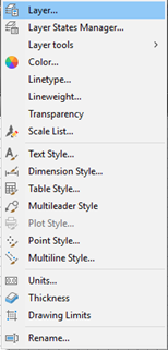
Fig. 3.1. Setting drawing limits
|
|
|
According to accepted terminology, these sizes are called drawing limits. Limits are a rectangular area of the XY plane, which is defined by two corner points - the lower left and upper right. Almost always, the point 0,0 is taken as the lower left corner - this is the default setting. When using the Advanced SetupWizard, it is assumed that the coordinates of the lower left corner are specified in this way, and therefore the width and the length are requested. After that, the installation of the Advanced Setup Wizard is considered complete and you can click Finish or Finish.
If the user has forgotten the sizes of the formats, then you can see them in the Print window (Fig. 3.2).

Fig. 3.2 Format Values in the Print Window
Work with layers
A feature of AutoCAD is the ability to work with layers. A complex drawing represents a set of layers, like tracing paper superimposed on top of each other. The main team working with layers is the Layer command. It displays the special dialog box Layer Properties Manager (Layer Properties Manager), in which you can both configure (change) the parameters of existing layers and create and configure the parameters of new layers (Fig.3.3).
You can invoke the Layer command in any of the standard ways:
- from the menu bar execute the command Format (Format) - Layer (Layer);
- click on the button of the toolbar Layers or on the Main tab of the tool ribbon (in the Layers group);
- enter in the command line: _layer (or LAYER).

Fig. 3.3 Accessing Layers in the Ribbon Interface
Create a new layer
To create a new layer, simply click on the button of the Layers toolbar or on the Main tab of the tool ribbon (in the Layers group). As a result, the Layer Properties Manager dialog box appears.
The Layer Manager window provides a list of all the layers in the drawing with an indication of their properties and parameters. By default, there is only one layer - a layer named 0. All information about the layers is presented in a table.
To create a new layer, in the Layer Properties Manager window, click on the New button at the top or right-click in the right half of the window and select the New command in the context menu that appears.
As a result, a layer with standard settings will be created and you will be asked to enter its name. By default, layers are named Layer 1, Layer2 (or Layer1, Layer2), etc. However, it is recommended to give layers more meaningful names.
Layer options
There are two ways to change layer parameters. The first way is to configure the parameters directly in the table itself, which contains information about the layers.
In this custom setting, click the left mouse button and the pop-up auxiliary window, select the required value.
To use the second method, you need to click the Show details button (details). In response to this, the bottom of the window will have additional controls, and through which are made the necessary settings.
In layer properties Manager will consider the parameters:
· Status (Status) — indicates the type of item: layer filter, layer used, empty layer, or current layer;
· Name (Name) - this field indicates the name of the layer. To change it, click on it with the left mouse button and type a different name;
· On (On) - this column shows the status of the layer: is set to On (On). on or off Off (Off). To change the status, click the mouse on the bulb which will then “light up”, then “fade”;
· Freeze (Freeze) - indicates the frozen or thawed layer. By default, each layer is thawed, as evidenced by the icon in the form of the sun. Clicking on this icon with the mouse, you will freeze the layer (is then the sun will be shown snowflake);
· To block (Lock) - here is the lock and unlock layers. Unlocked layers are indicated by an icon in the form of an open lock and a blocked - in the form of a padlock;
· Color (Color) - this column shows the color that will be used for all objects on this layer, whose properties as a color value is specified By layer (ByLayer);
· Type of line (Linetype) - set the line type for the layer. It will be used for all objects on a given layer, whose properties as the line type is specified By layer (ByLayer);
· Lineweight (Lineweight) - specifies the thickness of the line. This thickness will be used for all objects on a given layer, whose properties as the thickness is specified By layer (ByLayer);
· Transparency (Transparency) is a new feature introduced in AutoCAD 2012. Allows you to set the transparency of a layer, that is, how through the objects of the layer will show through the underlying layers. Value 0 - the layer is completely opaque, value 90 - maximum transparency;
· Print Style (Plot Style) - indicates the print (drawing) style of the layer;
· Print (Plot) - here you can set whether this layer will be printed when the drawing is printed or not. Layers for which the printer icon is set will be printed. If you click on this icon with the mouse, a prohibition icon will appear, and all constructions on the layer will not be printed.
· Frozen on new REs (Freeze ...) - allows you to freeze selected layers on new viewports.
Special settings
Setting the color .
To change the existing color value for a layer, in the Layer Properties Manager window, click on the corresponding square in the Color column. As a result, the Select Color dialog box opens. Having found a suitable color in this window, click on it with the mouse - and it will be selected. At the same time, a color usage pattern will appear at the bottom of the window, and the numerical equivalent of the color will be indicated next to the picture. Verbal names have only standard colors: yellow (yellow), cyan (cyan), red (red), green (green), blue (blue), white (white) and violet (magenta).
By the way, it is these colors that are recommended to be used in most cases, since they are the most different from each other.
Set line type.
By default, AutoCAD sets the line type to Continuous for all lines. To change this value and set the layer type to a different type, in the Layer Properties Manager window, in the line of the custom layer, click in the Linetype column. As a result, the Select Linetype dialog box appears, in which you can make your choice (Fig. 3.4). In this case, simply click on the desired value and click on the OK button.
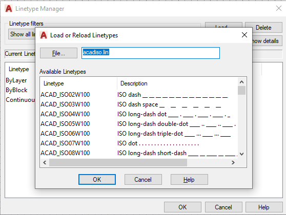
Fig. 3.4 Line Type Selection
If the set of options offered in the Select Linetype window does not contain the type you need (sometimes only one Continuous type is initially offered at all), then you should load other options in this window. To do this, click on the Load button. After that, the Load or Reload Linetypes window will appear.
Specifies the line thickness.
By default, in AutoCAD, all lines are drawn with a thickness of 0.010 inches, which is approximately equal to 0.25 mm. This value is usually conveyed by the word DEFAULT.
To set a different value for a particular layer, in the Layer Properties Manager window, click for this layer in the Lineweight column. Next, in the dialog that appears, select the desired value and click on the OK button.
Graphical user interface
After you have loaded the system, the AutoCAD 2017 graphic window will appear on the screen in the layout Drawing and AutoCAD annotations (Fig. 3.5).
|

|
|

|
|


Fig. 3.5 Line Type Selection
Four functional areas can be distinguished on the screen:
-a working graphic zone, in which the drawing is created directly, supplemented by pictograms of the coordinate system and a view cube;
-quick access panels;
-command line;
-status bar.
AutoCAD 2017 workspaces are Drawing and Annotations, 3D Fundamentals, and 3D Modeling (Figure 3.6). They demonstrate the so-called tape interface. The ribbon has eight tabs, the transition between which is carried out by clicking on their names above the tape itself.


Fig. 3.6. Kinds of tapes depending on the type of activity.
Using the system menu
At the very top of the screen is a title bar, similar to the title bar of any Windows application (it contains the name of the program, in our case, AutoCAD 2017, and the name of the current drawing). In the quick access panel, by clicking on the drop-down triangle, select Show menu bar (Fig. 3.7). We get the line of the falling menu (Fig. 3.8).

Figure 3.7. Activating the drop-down menu bar.

Figure 3.8. AutoCAD 2017 System Menu
The File menu, which includes all three types of items, is shown in Figure 3.9.


Fig. 3.9. An example of a menu that includes three types of items
The tape interface involves working with the following tabs:
- Home - this tab is available by default when AutoCAD 2017 starts and contains all the basic tools for drawing and editing, managing layers, inserting blocks and annotations, as well as setting properties of construction objects;
- Insert - designed to work with blocks and their attributes.
- Annotations - includes applying dimensions, editing annotations, working with tables and text labels;
- Parameterization - contains tools for defining geometric and dimensional dependencies, as well as managing existing dependencies in the drawing;
- View - contains settings that affect the parameters and methods of displaying the drawing in the AutoCAD 2017 window, as well as the appearance of the AutoCAD 2017 window itself.
- Management - contains tools for customizing the interface of the AutoCAD window for managing drawings and data;
- Conclusion - the tools for printing and export are concentrated on this tab.
Add-ons
A360
Recommended Apps
- BIM360
Performance.
Basic operations related to ease of drawing are called up with function keys. shows There are some function keys and their purpose in the table No. 1.
Table 1.
| Function keys | System action |
| F1 | Help call |
| F2 | Turn on / off the text box |
| FЗ | Turn on / off object snap mode |
| F5 | Switching isometric planes |
| F7 | Turn on / off grid mode |
| F8 | Turn on / off the ORTO mode |
| F9 | Turn on / off step |
| F10 | Turn polar polarization on / off |
| F11 | Turn on / off object tracking |
| F12 | Enable / disable dynamic input |
Tool palette
In addition to toolbars and toolbars, AutoCAD provides a tool palette (Figure 3.10.). It is designed to quickly place on the drawing the most commonly used blocks and hatchings. To display the palette tools, type “Ctrl” + “3” on the keyboard or select “Tool palettes” in the “View” tab of the ribbon.
In total, AutoCAD provides five methods for setting coordinates:
Interactive method.
Absolute coordinate method.
The method of relative rectangular coordinates.
The method of relative polar coordinates.
Setting the direction and distance.
Dynamic input
When creating and editing objects, it is convenient to use the dynamic input function. Using the dynamic input function, coordinate values can be entered not on the command line, but in the tooltip field, which is displayed next to the cursor and is dynamically updated as the cursor moves. The dynamic input function is turned on and off in the status bar (Fig. 3.11) using the F12 function key

Fig. 3.11. Status Bar Elements
If this function is enabled, next to the cursors information is displayed and dynamically updated as the cursor moves, the information displayed in the prompts as well as on the command line. When a command requires entering any parameters (length of a segment, circle radius, etc.), dynamic input fields are displayed. To select parameters (options) from the list, a special label is displayed in the dynamic tooltips indicating a list of such options. Having opened this list, you can select one of them. The procedure for entering coordinates in dynamic input fields
When the dynamic input function is turned on, several input fields are displayed next to the cursor crosshair, one of which is highlighted in blue (Fig. 3.12a). You can immediately enter data in this field. To go to the next field, click the Tab key on the keyboard. At the same time, a lock symbol appears in the field where the data has already been entered, indicating that this parameter has already been defined – (Fig. 3.12b).
To return to the field where the data was previously entered, click the Tab key again.


|
|
|

|


|
|
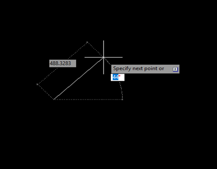
Figure 3.12. Display information of dynamic fields in various states:
a) displaying information of dynamic input fields before data has been entered into the field;
b) displaying information of dynamic input fields after data has been entered in the field.
Dynamic Input Function Assignment
The dynamic input function controls three components:
1. By entering the coordinates of the points in the dynamic input fields next to the crosshairs of the cursor.
2. Entering dimensions (in cases where this is possible).
3. The output of dynamic prompts with the ability to select them directly from these fields.
The user can enable or disable the output of individual components that are controlled in the Drawing Setting dialog box on the Dynamic Input tab.
Entering point coordinates in dynamic input fields
The coordinates of the points will be displayed in dynamic input fields if the Enable input with mouse checkbox is selected.
Depending on the settings specified in this window, the coordinates of points can be displayed in polar or Cartesian format and in absolute or relative coordinates.
Entering dimensions in dynamic input fields
To provide the possibility of entering dimensions into dynamic fields, in the Drawing Setting dialog box on the Dynamic Input tab, select the Enable dimension input box, where possible (Fig. 3.13). When this mode is enabled, dynamic dimension input fields are displayed next to the cursor crosshair.

Figure 3.13. Dynamic Input Tab of the Dialog Box
Drawing Modes (Drawing Setting) is designed to control the elements of the dynamic input function.
To configure the parameters of this mode, use the Dimension input parameters dialog box, which can be called up by the Settings button located in the Dimension input area (Fig. 3.13).
Depending on the settings for a given parameter, one, two or more user-defined size input fields may be displayed. You should not get carried away with displaying too many input fields.
By default, the Dimension Input Settings dialog box (see Figure 3.13) is set to display two input fields. This is usually enough for convenient editing of objects using this mode.
|

|
 a)
a) 

|
|

|
 b)
b) 
Figure 3.14. Output of dynamic dimension fields for created objects:
a) the output of dynamic input fields for dimensions when creating a circle;
b) output of dynamic input fields of dimensions when creating segments.
Laboratory work.
Binding Features
The use of a pointing device for precise input of coordinates requires the use of special commands:
• SNAP step-by-step binding - coordinates to the nodes of an invisible grid;
• OSNAP object snap - object snap - coordinate snap to various points of already created objects.
Step binding. The SNAP command allows you to snap all points to nodes of an imaginary grid with a user-defined step. This grid can be made visible using the GRID command. The presence of the grid allows you to quickly evaluate the sizes of fragments of the details of the drawing. In addition, potential snap points immediately become visible, although the pitch of the auxiliary grid visible on the screen does not have to coincide with the snap grid. Once you set the snap mode, the graphic cursor will only move between the nodes of the grid. You can adjust the snap characteristics in the Drafting Settings dialog box, the Step and Grid tab (Fig. 3.14). There are three ways to open a window:
 - using the Tools menu in the classic workspace Drawing modes;
- use the mouse to move the cursor to the Step link button located in the status line and select Settings with the right button.
- using the function key F9.

Figure 3.15. The Drafting Settings dialog box
Step and grid tab (Snap and Grid)
It is desirable that the grid pitch in all cases coincides on both axes. Then, when changing the value of the interval along the X axis, the system will automatically adjust the setting of the interval along the Y axis.
Using the Step and grid tabs is necessary when working with isometric constructions. For example, in laboratory and laboratory work volumetric parts should be built on a plane. We use the type of binding - Isometric. We turn on the ORTO mode and build the object, changing the isometry plane with the F5 function key.
Object snap . When entering points, you can use the geometry of the objects available in the drawing. In AutoCAD 2017, this method is called OSNAP object snap. It allows you to set new points relative to the characteristic points of existing ones.
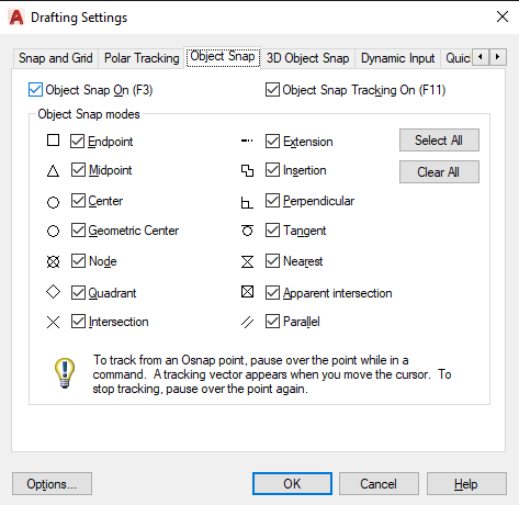
Fig. 3.16. Context menu for selecting the object snap mode
geometric objects. Object snap control is carried out from the Drawing Modes dialog box, Object Snap tab (Fig. 3.16) in the following ways:
• using the Tools menu in a classic workspace Drawing modes;
• use the mouse to move the cursor to the Step-by-Step button located in the status line and right-click to select Settings.
• using the function key F3;
• using the context menu (Fig. 3.16), which is called by clicking the right mouse button while holding down the Shift key.

Fig. 3.17. Object snap tab
It allows you to simplify all operations related to object snap. When the graphic cursor passes near a user-defined point, the system notifies you as follows:
- the point is marked with a marker, the shape of which depends on the type of snap and the point closest to the cursor;
- a contextual snap prompt appears near the point;
- the graphic cursor “magnetizes” to the found point.
Table 2 lists the options for object snap commands.
One of the most significant features that make it much easier to work in AutoCAD is AutoSnap.
Table 2
Object snap command options
| Option | System action |
| Point | Snap to the closest endpoint of a line or arc, multiline, area border and three-dimensional body |
| Mid | Midpoint of objects such as line, arc, multiline |
| Intersection | The intersection of two lines, a line with an arc or circle, two circles and / or arcs, splines, area boundaries |
| Continuation | The function of binding to the continuation of objects. Helps the user build objects based on lines that are temporary extensions to existing lines and arcs |
| In the center | circumference |
| Quadrant | Snap to the nearest quadrant point on an arc, circle, or ellipse |
| Tangent | Snap to a point on a circle or arc that, when connected to the last point, forms a tangent |
| Normal | Snap to a point on a line, circle, ellipse, spline or arc, which together with the last point forms a normal to this object |
| Parallel | The function of binding objects to parallels, which expands the possibilities of constructing objects parallel to existing ones |
| Insertion point | Snap to insertion point of text, attribute, form, attribute or block definition |
| The nearest | Snap to a point on a line, arc, or circle that is closest to the position of the crosshair |
Дата добавления: 2020-04-25; просмотров: 143; Мы поможем в написании вашей работы! |

Мы поможем в написании ваших работ!