Life at uniaxial static tension
To determine the time before fracture, the exponential equation below is commonly used
 .
.
This equation is based on the thermofluctuation theory for highelastic materials, it's described in Russian Standards, thermal part of it is [2]. For calculation simplicity, the logarithmic form of exponential equation is as shown below
 (3.1)
(3.1)

The equation (3.1) is well coordinated to experimental data, when the rubber is in a high-elastic state. That is at temperatures higher glass transition temperature, that practically covers operation at temperature range.
To determine the indispensable constants (b, Uo, lgC), the experiments of uniaxial load of dumbbells is used (more details in the next section).
Application range of the equation (3.1): static load; the dominating value in a tensor of the first principal stress (this value also will be used in (3.1)); temperature range from glass transition temperature up to temperature of thermodestruction; lower limit of experimental time 300 seconds. It is recommended to use when problem solving of uniaxial tension, torsion and shear, deforming of membranes.
Life at complex static stressed state
In case of a complex stress, the lifetime depends on stresses tensor components. From the physical point of view, the energy of activation U of fracture of the stretched bonds in material as a scalar should depend on an invariant components of a tensor of stresses.
Stretching strains, which give rise to fracture, are connected with deviator stress component. In linear elasticity  . For elastomers characterized by constant volume at deforming, deviators of strains equal to itself. To determine the lifetime in a complex - stress of state
  is used.
Fixing the contribution of tensile stresses (  ) in process of fracture, it is possible to note as evidence experimentally fact of lifetime increasing when pressure is applied. The pressure slows down the effect of tension in progressing fracture. The experimental data obtained on rigid polymer, were well interpolated by equation
  with relationship
  . For elastomers in a high-elastic state the exponential relation of lifetime on tensile stresses is maintained. The energy of activation is presented in the form
  , where empirical coefficient, takes in to consideration, the contribution of mean stresses or hydrostatic pressures in variation of speed of fracture.
Summing up what has been said told, the relationship for prediction will look as
|
|
|
 . (3.2)
The difference from (3.1) is, that first principal deviator stresses multiplied by 1.5 is used. Coefficient a in equation (3.2) is determined by processing data of tensile failure of dumbbells in conditions of the additional pressure applied. These experiments are expensive, therefore from the practical point of view the experiments of fracture of cylindrical samples at contraction are move worth.
Life of compressed cylinders
The right approach for analysis of lifetime in state of the complex stress is the experiments for determination of long strength of cylindrical samples at contraction. The results of experiments are used for two purposes. First – checking of the applicability of the formula (3.2) and parameters b, Uo, lg C, obtained from tension of dumbbells experiments, in the case of state of the complex – stress. Second – determining of the parameter  .
.
When contraction of the free cylinder, its ends are not fixed, it is necessary to lower the frictional coefficient at ends. For example, lubricate with inert silicone oil the chromium-plated polished surface of plates. The frictional coefficient is reduced to 0.01  0.03.
0.03.

Fig. 3.3
During experiment, the cylinder is loaded with constant load F at temperature T = 20 °C = 293 K. The time before appearance of the first fractures is fixed. The place of their occurrence and directions depend on many factors: type of rubber, magnitude of friction, shape of the cylinder, level of loading. During experiments cylinders made of elastomer E50189 different shape were taken into consideration. For these shapes two types of fracture were observed on a surfaces perpendicularly to circular coordinate (Fig. 3.3, а) and inside the cylinder perpendicularly to radius (Fig. 3.3, b).
The first cylinder with do = ho = 10 mm fractured when contraction force F ³ 18.5 kN at 390 ± 100 sec. (6.5 min.) was applied. Fracture started at the field point E (Fig. 3.4). Cracks appeared on surfaces and spread perpendicularly to direction .
|
|
|
On free surfaces hydrostatic pressure is equal to zero i.e.  . The magnitude of parameter a does not have any value. For this rubber other values are determined (detail these in next section). This allows calculate Lifetime in this point. The field of the first principal deviator of stresses is shown in Fig. 3.4. At point E is
  .
.
The coinciding of magnitudes of lifetime shows that, for prediction of surface fracture and in complex cases it is enough to obtained constants of relationship (3.2) from uniaxial tensional results. To obtain the constants describing hyper-elastic behavior of material (about this see the next section) and calculate principal deviator stress  in a part. Then, use the relationship (3.2) for prediction.
In other points, deviator stresses are higher, but they are partially suppressed by hydrostatic pressure. At internal point I:  ,
,  .
.
The second cylinder do = 28.6 mm, ho = 12.5 mm fractured when contraction force F = 115 kN at 420 ± 100 seс. (7 min, lg  = 2.63). Fracture always started at point I and spread perpendicularly to direction r. They can only be seen after cutting through a fractured sample.
Point I is internal. At this point hydrostatic pressure is  . To calculate of lifetime at internal points, it is necessary to know magnitude of a. In this case we have a inverse task: knowing lifetime to determine a. From the formula (3.2) we will obtain
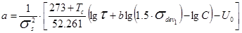 . (3.3)
The first principal deviator stress field is shown in Fig. 3.5. At point I:  . Putting these values in (3.3), for compound we will obtain

Knowing all values included in the formula (3.2), it is possible to calculate lifetime not only on edge of the cylinder, but also inside it. The lifetime field for the first cylinder is shown in Fig. 3.6. The zone of minimal lifetime as before is on lateral surface of the cylinder.

Fig. 3.4
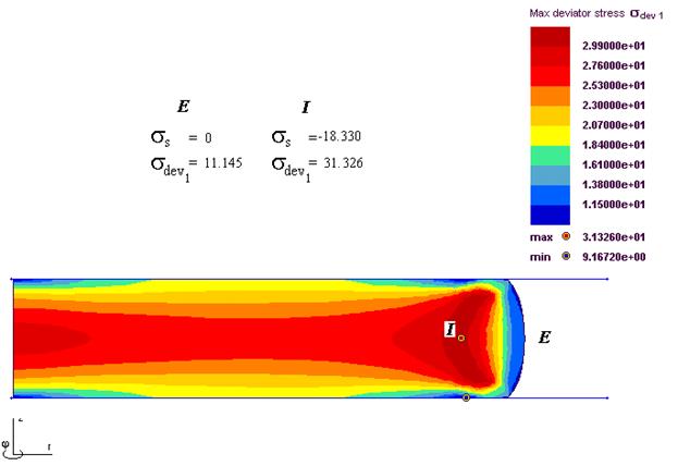
Fig. 3.5

Fig. 3.6
Дата добавления: 2019-09-13; просмотров: 159; Мы поможем в написании вашей работы! |

Мы поможем в написании ваших работ!