On the homeostat. In S.5/14 (which the reader should read again) we
Considered it as a whole which moved to an equilibrium, but there
We considered the values on the stepping-switches to be soldered
On, given, and known. Thus B’s behaviour was determinate. We
Can, however, re- define the homeostat to include the process by
233
 A N I N T R O D UC T I O N T O C Y B E R NE T I C S
TH E ERR O R- CO N TR O LLED REG U LA TO R
Which the values in Fisher and Yates’ Table of Random Numbers
Acted as determinants (as they certainly did). If now we ignore (i.e.
Take for granted) the resistors on the switches, then we can regard
Part B (of S.5/14) as being composed of a relay and a channel only,
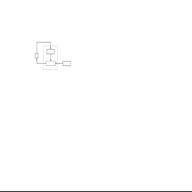
To which comes values from the Table. We now regard B as having
Two inputs.
B
Relay
A
Channel
Table
B’s state is still a vector of two components— a value provided by
The Table and the state of the relay (whether energised or not). To
An Observer who cannot observe the Table, B is Markovian (com-
pare S.12/9). Its input from A has two states, β and γ; and it has been
built so that at β no state is equilibrial, and at γ every state is. Finally
It is coupled as in S.5/14.
The whole is now Markovian (so long as the Table is not
Observed). It goes to an equilibrium (as in S.5/14), but will now
Seem, to this Observer, to proceed to it by the process of hunt and
Stick, searching apparently at random for what it wants, and
Retaining it when it gets it.
It is worth noticing that while the relay’s input is at β, variety in
The Table is transmitted to A, but when the input comes to y, the
Transmission is stopped. The relay thus acts as a “tap” to the flow
Of variety from the Table to A. The whole moves to a state of equi-
Librium, which must be one in which the entry of variety from the
Table is blocked. It has now gone to a state such that the entry of
Variety from the Table (which would displace it from the state) is
Prevented. Thus the whole is, as it were, self-locking in this con-
Dition. (It thus exemplifies the thesis of S.4/22.)
The example of the previous section showed regulation
Occurring in a system that is part determinate (the interactions
Between the magnets in A) and part Markovian (the values taken by
The channel in part B). The example shows the essential uniformity
And generality of the concepts used. Later we shall want to use this
234
Generality freely, so that often we shall not need to make the distinc-
Tion between determinate and Markovian.
Another example of regulation by a Markovian system is worth
Considering as it is so well known. Children play a game called
“Hot or Cold?” One player (call him Tom for T) is blindfolded.
The others then place some object in one of a variety of places,
And thus initiate the disturbance D. Tom can use his hands to find
The object, and tries to find it, but the outcome is apt to be failure.
The process is usually made regulatory by the partnership of Rob
(for R), who sees where the object is (input from D) and who can
Give information to Tom. He does this with the convention that
The object is emitting heat, and he informs Tom of how this would
Be felt by Tom: “You’re freezing; still freezing; getting a little
warmer; no, you’re getting cold again; …”. And the children (if
Young) are delighted to find that this process is actually regula-
Tory, in that Tom is always brought finally to the goal.
Here, of course, it is Tom who is Markovian, for he wanders, at
Each next step, somewhat at random. Rob’s behaviour is more
Determinate, for he aims at giving an accurate coding of the rela-
Tive position.
Regulation that uses Markovian machinery can therefore now
Be regarded as familiar and ordinary.
DET ER M I NATE R EGUL ATI ON
Having treated the case in which T and R are embodied in
Дата добавления: 2019-11-16; просмотров: 301; Мы поможем в написании вашей работы! |

Мы поможем в написании ваших работ!