WAVE FORMATION FACTORS. CALCULATION OF WAVES ELEMENTS WITHIN THE OPENED WATER AREAS
THE MINISTRY OF SCIENCE AND HIGHER EDUCATION OF THE RUSSIAN FEDERATION
Far Eastern Federal University
School of Engineering
CALCULATION OF WAVES ELEMENTS WITHIN WATER AREAS
Training Electronic Edition
Methodical recommendations for practical trainings and master thesis
Majoring 08.04.01 Construction
Vladivostok
Far Eastern Federal University
2017
UDK 627.042(083.75)
Sabodash, О.А., Seliverstov, V.I. Calculation of waves elements within water areas / O. A. Sabodash; V. I. Seliverstov [Electronic Resource] / Engineering School FEFU. - Electronic data - Vladivostok Far Eastern Federal University, 2017 [45 p.]. – 1 CD-ROM. - System requirements: processor speed 1.3 GHz (Intel; AMD); operating memory 256 MB; Windows (XP; Vista; 7; etc.); Acrobat Reader, Foxit Reader or analog.
Methodical recommendations are prepared in compliance with "Shelf and Port Equipment" and "Shelf and Coastal Construction" disciplines program developed as per the instructions of Federal State Educational Institution of Higher Professional Training majoring 08.04.01 Construction (Magistracy). Methodical recommendations include basic definitions on wind waves and its particulars, brief description of wave’s formation factors and its definitions, calculations of wind wave’s elements for open and closed water areas.
Methodical recommendations are intended for bachelors, masters, postgraduate students studying the construction of marine hydrotechnical structures and continental shelf structures, inclusive of teachers and designers, technologists, constructors and operators.
Key words: waves; wind; water area; deep water area; shallow area; coastal area; refraction; diffraction; transformation; probability.
Editor G. B. Arbatskaya
Design and positioning N. O. Kovtun, G. P. Pisareva
Published:
PDF format
Size ___ MB [4, 9 ref.print.pages ]
Quantity (100 copies);
Methodical recommendations are prepared by the editing and publishing department of FEFU Engineering School
[Russian Island, Ayaks Settlement; 10 12 building, FEFU Engineering School, Editing and Publishing Department, office С 714]
Far Eastern Federal University
690950, Vladivostok, Russia 8 Sukhanova Str.
CD-ROM manufacturer: The Direction of Publishing Activity
690950, Vladivostok, Russia 10 Pushkinskaya Street
©Sabodash O. A., 2017
|
|
|
© FSAEI of HE «FEFU», 2017
INTRODUCTION
Wind waves within seas and water-storage reservoirs are formed due to friction force and complex interaction between air flow (wind) and water. Heights and lengths of waves can be significant; force impact of waves for several types of hydrotechnical structures (protective; beaching) can prevail upon the other types of load. So, any knowledge on wind waves and its impact is necessary for development of hydrotechnical structures.
In order to define wave impact upon structures and to evaluate the protection level for water areas, it is necessary to obtain the calculating values for basic wave’s elements, i.e. height, length and period.
The process of formation and development of wind waves is rather complicated. There are a lot of factors influencing wave’s parameters and type inclusive of velocity, direction and evenness of wind, size and configuration of water surface, water depth, bottom configuration, etc.
BASIC TERMS AND DEFINITIONS
Several basic terms related to wind waves are used herein.
1.1. Wave profile and elements
Wave profile is an intersection of wave surface and vertical plane corresponding to wave development direction (see Fig. 1.1). The following definitions are related to the profile:
AVERAGE WAVE LINE – means a line that is crossing the wave vibration record so, that the total area above or under this line can be calculated as follows: for regular wave - the horizontal line within the half-sum level of its upper and lower elevations: the rise of average wave line above the remaining level shall be defined as follows:
For traveling waves  , (1.1)
For standing waves:  , (1.2)
|
|
|
where h and λ means height and length of traveling wave correspondingly;
H – water depth;
WAVE CREST – means wave area located above the average wave line;
WAVE HOLLOW – means wave area located under the average wave line;
WAVE TOP – means the highest point of wave crest;
WAVE BOTTOM – means the lowest point of wave crest;
WAVE SURFACE – means a line within the plane of disturbed surface located at the crest top of corresponding wave;
WAVE LINE – means a line that is perpendicular to wave surface within this point (wave development direction).
The basic elements of wave are as follows (see Fig. 1.1):
WAVE HEIGHT h – exceeding of wave top in relation to next bottom of wave profile;
|
|
|
|
|
|
|
|
|
|
|
|
|
|

Figure 1.1 Wave profile.
WAVE LENGTH λ – means horizontal distance between top of two adjacent crests of wave profile;
WAVE PERIOD τ – means the time of passage for two adjacent tops within the fixed area;
 (1.3)
(1.3)
The following terms are used:
WAVE SLOPE – means relation of wave height to its length h:λ;
WAVE FLATNESS – means value that is inversive to wave slope λ:h; relative wave slope α and relative water depth β:

 (1.4)
(1.4)
WAVE FREQUENCY  and WAVE NUMBER k :


 ;
; 
 (1.5)
(1.5)
WAVE DEVELOPMENT VELOCITY с – means the velocity of wave crest movement subject to development direction:
 (1.6)
(1.6)
|
|
|
1.2. Rated wave elements
The intensity of waves within the water area depends from different factors. Maximum wave elements and maximum wave load acting upon structure usually occurs during storm featured with the strongest winds. It is obvious that in case of ports and hydrotechnical structures design, loads shall be defined with due consideration of wave influence formed subject to storm with definite force. So, the term of rated storm shall be considered.
Rated storm – is a storm with intensive wind heave once per defined number of years nt. The intensity of heave is assumed by the average height of waves  . Structure permanentness class depends upon the structure responsibility, i.e. the highest rated storm shall be considered (with less repeatability).
Repeatability of calculated storm – means the value that is inversive to the defined number of years nt , subject to one rated storm for this period. The higher structure permanentness class, the smaller repeatability of rated storm (see Table 1.1).
Table 1.1
Calculated values of repeatability and cumulative probability of rated storm
| Structure class | nt, years | Repeatability of rated storm 
| Cumulative probability of rated storm, % |
| I and II | 50 | 0.02 | 2 |
| III and IV | 25 | 0.04 | 4 |
Cumulative probability of rated storm means the number of storms with defined force, specified in per cent (rated storm) during 100 years. For example, if the rated storm can occur once per 25 years (nt=25 years), so the cumulative probability of rated storm will be equal to 4%; moreover, for the most responsible hydrotechnical structures the cumulative probability of rated storm can be equal to 1%.
Wind waves formed within the water area are irregular. If we consider several sequential waves (for example, in case of rated storm), so we will find that each of these waves is featured with different elements (length, height, period) that are different from corresponding elements of the other waves.
Rated height of wave
Rated height of wave means the wave height subject to cumulative capability for this system. Cumulative capability of wave height for wave system means the number of waves from one hundred sequential waves (in case of rated storm) with the same or higher height. For example, there are five 5.5 m or higher waves among 100 sequential waves. It means that the cumulative capability of 5.5 m wave for this system is equal to 5%. Once there are two waves with 6 m or higher among 100 sequential waves, so the cumulative capability of 6 m waves for this system will be equal to 2%.
|
|
|
Values of rated cumulative capability of waves for system subject to marine hydrotechnical construction shall be defined in compliance with Table 1.1. Calculation of heights to another cumulative capability or average height h of waves to hi wave with i-th cumulative capability shall correspond to item 2.1.
Calculated length and period of waves. An average length of wave shall be considered as a rated value  . As of penetrated structures, maximum wave impact for measurement of wave length is defined from 0.8 up to 1.4 , providing the highest value of wave load acting upon structure. Where is an average length of waves considering 100 waves system subject to the rated storm.
Rated period of waves τ shall be defined via rated length of waves λ using (1.3).
1.3 Rated water levels
Force impact of waves acting upon structure depends from wave elements value and from water level. There are fluctuation of level within the water areas due to piling up or down of water, tidal effects, etc. Rated level shall be defined for design purposes, i.e. water level for determination of force impact of waves inclusive of elevations and dimensions of structure.
Table 1.2
Values of rated cumulative probability i for wave height per system [1]
| No. Item | Application purpose | Cumulative probability i, % | Specific Notes |
| 1 | Stability and strength of HTS | ||
| 1.1 | Vertical profile | 1 | |
| 1.2 | Inclined profile with fencing: concrete slabs rubblework, standard or molded blocks | 1 |
|
| 2 | |||
| 1.3 | Transparent structures and single supports I class II class III, IV class |
| |
| 1 | |||
| 5 | |||
| 13 | |||
| 1.4 | Shore protection I,II class III,IV class |
| |
| 1 | |||
| 5 | |||
| 1.5 | Anchored floating structures | 5 | |
| 2 | Identification of port water areas safety | 5 | |
| 3 | Identification of wave surge | 1 | |
| 4 | Elevations of transparent structures | 0.1 | subject to corresponding justification |
Maximum rated level of water shall be defined as per SNiP requirements for designed structures [1]. For identification of loads and impacts acting upon hydrotechnical structures, the cumulative probability of rated level shall not exceed as follows: I class structures - 1% (once per 100 years); II and III class - 25% (once per 20 years); IV class - 10% (1 per 10 years) in compliance with the highest annual levels for ice-free period.
For shore protection structures the cumulative probability of rated level shall be assumed as follows:
as per the highest annual levels - support gravitational type walls (wave protection) II class - 1%; III class - 25% for artificial beaches with protective structures (dam dikes; underwater breakwaters IV class) - 50%.
The statistical data (maximum water level for calculated point) for 25 years are used in order to define the rated level. Application of such measurements can be assumed for less period subject to long-term observations of nearby areas.
Level of Z rise over average multi-year value can be assumed as a rated level for preliminary evaluating calculations:
 , (1.7)
where А – value of syzygial tide (tide less seas А = 0);
∆hset – height of wind surge
А value shall be defined in compliance with field studies using measurement data for nearby areas. The height of wind surge ∆hset shall be defined in compliance with field studies or using (without consideration of coastal line configuration; subject to permanent depth H) the following formula due to the absence of corresponding data
 , (1.8)
where a w - angle between water area axis and wind direction, degrees;
W - rated wind velocity, m/s;
D - acceleration, m;
Kw - index as per Table 1.3.
Table 1.3
Dependence of Kw index from wind velocity
| W m/s | 20 | 30 | 40 | 50 |
| Kw *106 | 2.1 | 3.0 | 3.9 | 4.8 |
Elevations of structures shall be defined subject to the cumulative probability for maximum water level and maximum wind speed.
1.4 Waves transformation next to shore
The diagram of wave’s transformation next to shore is shown on Fig. 1.2.
|
|
|
|

Fig. 1.2 - The diagram of wave’s transformation at shoaling waters:
1-1 – section of the first wave falling; 2-2 – section of the latest wave falling
Four zones can be identified:
ZONE 1 (deep water) with depth  ZONE 2 (shallow water) with depth
  ; ZONE 3 (surfing area) with depth
  ; ZONE 4 (pre-coastal area) with depth
  . Where H - water depth for considered section;
  - means average wave length for deep water area; Hkp – means critical depth for the first wave falling; «r» index means wave elements within the deep water area; upper line means an average value of wave elements. Zone 1 and 2 are featured with traveling waves. Wave’s transformation is started from depth
  . Shallow area waves (zone 2) are featured with less length, other height and water particles path in comparison with zone 1 (deep water area - circle).
Once water depth is decreased up to Hкp, surfy waves featured with dissymmetry and crest falling are formed. Than waves are crashed within the coastal line of zone 4 providing the progressive water streams.
WAVE FORMATION FACTORS. CALCULATION OF WAVES ELEMENTS WITHIN THE OPENED WATER AREAS
There are simple and complex conditions of wave formation. Simple conditions are related to simple configuration of shore and uniform wind velocity. Complex conditions of wave formation provide the difficult configuration of coastal line or inhomogenuity of wind velocity.
2.1 Identification of wave’s elements subject to simple conditions of wave’s formation
Water area with simple configuration, i.e. where the relation of the longest and the shortest beam for section  subject to the rated wind direction (up to opposite coast, island, etc.) is less than two. No obstacles are considered. Angle dimension is less than 25.50. Wind field shall be considered as homogeneous, once its velocity subject to fixed moment within the water area depth is the same (maximum difference 5 m/s).
Calculated elements of wind waves shall be defined subject to wind velocity  of rated storm with t duration of wind activity of rated storm subject to D acceleration and water area depth H.
W wind velocity for the rated storm. W value is defined via the statistical processing of multi-years observations data. Summary data on winds are published by various data books. The maximum observed velocity for this period related to the wave-hazard direction shall be considered as a rated velocity of wind, once complete wind data for nt period is available.
Rated wind velocity shall be defined using the probability table (see Figure 2.1), once multi-year periodical wind observations less than nt period is available.
Probability paper is the graphical dependency F=f(W) , where F – cumulative frequency of wind velocity for such point, %; W – wind velocity, m/s.

Fig.2.1 Diagram of probability
Cumulative frequency F is a relation of measuring number featured with less or equal velocity to the general number of performed measuring.
Probability paper shall be developed for each wave coast. It has the following purpose. As no time measurement data is sufficient, so rated velocity shall be defined using extrapolation method (extrapolation means the identification of function values out of defined interval using several known parameters). The task is to construct the probability line providing the dependence of integral repeatability F (%) from wind velocity subject to this rhomb line and to define rated storm wind velocity W as an abscissa for some point on this line (see below).
Points for development of line on the probability paper shall be identified as follows. Several points of wind velocity shall be marked on abscissa axis subject to the defined velocity. Than according to defined points the line shall be constructed within the probability table; rated storm wind velocity W shall be defined as an abscissa of point at the line subject to the integral wind repeatability, i.e. [1]:
 (%), (2.1)
where t – time of rated storm activity, hour. (see below); N - number of measuring for ice free year; nt – rated number of years (table 1.1); р – the repeatability of this wave-hazard direction of wind among the other directions shown as fractions.
Data on wind measurement for most areas of our country inclusive of coastal line is given in USSR Climate Reference Book [3].
Wind velocity data given in [3] was obtained via measurement of wind velocity using wind vane. Anemometer data (wind velocity W) are used for calculation of wave elements.
Moreover, once wind velocity is measured above the sea level Z≠10, so it shall be recalculated. Rated velocity of wind for 10 m height above the water area surface W, m/s, shall be defined as follows:
W=kfkzwz , (2.2)
where wz - wind velocity at 10 m from the ground (water area) surface, corresponding to 10 minutes averaged interval as per table 1.1; kz – wind velocity coefficient subject to water surface conditions for water areas up to 20 km assumed as follows: unit subject to measurement of wz wind velocity above water surface, above sand (coast, etc.) or snow areas; as per table 2.1 - in case of wind velocity measurement above A, B or C areas in compliance with SNiP requirements for wind loads [5]; kf – data calculation coefficient for wind velocity defined using wind vane as follows: kf = 0.675 + 45/Wz , but less than 1.
Wind action duration t. T value shall be defined on the basis of statistical data of observations for ice-free periods. Once no data is available, so t value can be considered as [1]: water storage reservoir and lakes – 6 hours, sea – 12 hours, oceans – 18 hours.
Table 2.1
Index kz subject to location
| Wind velocity Wz, m/s | А | В | С |
| 10 | 1.1 | 1.3 | 1.47 |
| 15 | 1.1 | 1.28 | 1.44 |
| 20 | 1.09 | 1.28 | 1.42 |
| 25 | 1.09 | 1.25 | 1.39 |
| 30 | 1.09 | 1.24 | 1.38 |
| 35 | 1.09 | 1.22 | 1.36 |
| 40 | 1.08 | 1.21 | 1.34 |
Wave acceleration D. D value shall be defined using maps for each wave course as a distance from the opposite coast, ice area or storm zone border up to this point. Acceleration shall be defined against wind. Different acceleration shall be assumed for each wave dangerous direction.
For the further identification of wave elements, an average value of acceleration (m) for defined rated wind velocity W, m/s, shall be calculated as follows:
 , (2.3)
where k – coefficient equal to 5*1011 ;  - kinematic viscosity equal to 10-5 m2/s.
Value of maximum acceleration Dn , m, shall be defined as per Table 2.2 for assigned rated wind velocity W, m/s.
Table 2.2
Maximum acceleration Dn subject to defined rated wind velocity W, m/s
| Wind velocity W, m/s | 20 | 25 | 30 | 40 | 50 |
| Maximum acceleration Dn 10-3, m | 1600 | 1200 | 600 | 200 | 100 |
Definition of wave elements within deep water and shallow areas (water areas) Average height  and period
  of waves shall be defined as per the diagram on Figure 2.2. For deep water area (or zone ) the upper curve is used; for shallow area (shallow area with bottom incline 0.001 or less) – curves with corresponding value of gH/W2.
Identification of values  and
and  subject to known t, W, D shall be performed as follows (see Figure 2.2). Nondimentional ratios gt/W and gD/W2 are calculated, i.e. to be shown as x-coordinate (moreover, axis gt/W is moved down). Once the defined point on gt/W axis is located to the left from corresponding point on gD/W2 axis, so sea is considered as developed, otherwise it shall be considered as stable. In case of developed sea the gt/W axis is used; axis gD/W2 is used for stable sea.
Once the type of sea is defined (stable or developed), so the points gt/W or gD/W2 for the corresponding curve subject to defined value gH/W shall be obtained. Further ordinates for these points shall be defined (subject to displacement). In compliance with obtained  and
and 
 values, and
  can be defined. The line of and
  values identification shown by the dotted line on Figure 2.2.
An average length of waves  deep water
  ) shall be defined as follows [1]:
 2 (2.4)
For shallow water area the dependency between  and
and  is shown on Figure 2.3.
Wave height hi with i-th probability ratio can be defined, once an average height of wind waves is defined. Rated values of cumulative probability shall be assumed with due consideration of structure class and type as per Table 1.2. hi value shall be calculated as follows:
 , (2.5)
where ki - transformation index.
The value of ki coefficient shall be defined as per the diagram on Figure 2.4. As for the deep water areas, X-axis gD/W2 shall be used. Axis, located to the left from corresponding values on the other axis among gD/W2 and gН/W2 shall be used for shallow water areas.
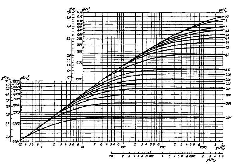
Figure 2.2 Diagram for identification of wind waves elements at deep water and shallow areas
2.2 Identification of waves elements subject to complex conditions of waves formation
Wave elements depend upon several factors inclusive of coastal line configuration and inhomogeneity of wind velocity. Usually one or both factors shall be considered.
An average height of wave subject to complex configuration of coastal line (without consideration of inhomogeneity of wind velocity) shall be calculated as follows [2]:
 , (2.6)
where  , m for (n=0;±1; ±2; ±3;) – average height of wave, in compliance with figure 2.2 subject to the rated velocity of wind and beams view Dn, m for direction of main beam and wind direction. Beams shall be shown from rated point up to crossing with coastal line with 22.5° interval from the main beam.
An average period of waves shall be defined subject to size-less value , as per Figure 2.2. considering known size-less value , an average length of waves shall be defined as per (2.4) formula.
Weather charts shall be used for accounting of wind velocity inhomogeneity. Wind velocity shall be defined using the gradient of atmospheric pressure, width of rated point, and difference of air temperature, etc.

Figure 2.3 Dependence between wave period and length for shallow area

Figure 2.4 Diagram of ki coefficient for wave calculation with i-th cumulative probability.
2.3 Identification of transformed waves elements
In case of waves distribution from deep water area to shallow area, i.e. to coastal line subject to decrease of depth, the phenomena of transformation and refraction is accompanied by energy loss. Height and length of wave are changed, but the period stays constant.
Wave transformation – means the phenomena of wave profile transformation and wave elements change in case of shoaling waters due to the bottom influence.
Wave refraction – means the phenomena of wave turn in parallel to sea contour due to the dependence of wave development velocity from depth.
The influence of transformation and refraction upon wave elements shall be considered separately subject to the application of corresponding coefficients.
The height of transformed wave with i-th cumulative probability within the shallow area subject to 0.002 bottom incline shall be defined as follows:
 , (2.7)
where kr – coefficient of transformed wave;  - wave refraction coefficient;
  - average coefficient of loss;
  - height of initial wave with i%-th cumulative probability.
The height of initial i%-th cumulative probability  : for deep water areas it is equal to wave height subject to
  , for shallow areas is equal to wave height subject to depth decrease.
Transformation coefficient  for formula (2.4) shall be defined in compliance with Figure 2.5 as an ordinate (left axis) for point with abscissa
  (where Н – is a depth of water for considered area).
Refraction coefficient shall be defined using the refraction plan. Refraction plan means the plan of water area with wave beams. See Figure 2.6 for development inclusive of legend for corresponding diagrams.
The example of refraction plan development is shown on Figure 2.6. Previously parallel beams are shown on water area plan (distance between beams (1÷2) ). Each beam of refraction plan shall be formed separately. Beam curving is started from isobaths  . Depending from angle αi of beam approach to i-1 isobaths, inclusive of relation for the next isobaths i-1 as per Figure 2.6, angle
  of beam deviation from the initial direction shall be defined. Cross point of this beam and isobaths provides wave beam point with consideration of refraction. Then, considering the angle between the new direction of beam and i-1 isobaths , for i-1 and i-2 isobaths, new parameter of wave beam deviation shall be defined, etc.
The construction shall be up to the border of designed structure, but less than the inshore area.
Once wave beam and isobaths are almost parallel (α>80°), so no above mentioned method can be applied due to the significant decrease of accuracy. The sequence of identification of rotation angle Dαi of wave beam shall be as follows: The interval between isobaths shall be subdivided by transverse lines for several sections (see Figure 2.7). The distance between section borders R shall be divisible for distance between J isobaths for this section. Wave crest velocity for considered isobaths shall be defined as follows:
 , (2.8)
where H – isobaths depth, m; k – wave value
For correlation of isobaths velocity  and size-less correlation
  , the angle of beam turning shall be defined for each diagram on Figure 2.8. The beam shall be drawn up to the middle of section subject to turn for
  . It shall be repeated up to the moment when α will become less than 80°.
Refraction coefficient kр for (2.7) is equal to
 , (2.9)
where S0 – is a distance between two adjacent deep water beams at the refraction plan; S – is the shortest distance between the same beams at the refraction plan regarding calculated point.
Generalized coefficient of losses kп shall be defined as per Table 2.3 with due consideration of i bottom incline and relation value .
Length of transformed wave. The length of transformed wave shall be defined as per Figure 2.9 subject to defined adjustable values and  . Wave period is equal to deep water area period.
Wave top shall be calculated  in compliance with the rated level as per Figure 2.10 subject to and
  .
.

Figure 2.5 Diagram for identification of transformation coefficient and critical depth.
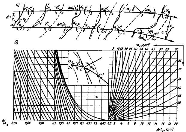
Figure 2.6 Diagram for refraction plan development.

Figure 2.7 Construction of diffracted wave beam considering α>80°.

Figure 2.8 Dependence of angular deflection from 
Critical depthНкр. Critical depth subject to first falling shall be defined for assumed bottom incline as per diagrams 2,3 and 4 on Figure 2.5 for each value and Figure 2.5 using the method of progressive approximation.
For several depth Н using formula (2.7)  , shall be defined, than using diagram 2.3 and 4 on Figure 2.5 for each parameter
  fined
fined  and defined Нкр, applying those Нкр, matching with one of applied depth Н.
Table 2.3
Generalized coefficient of losses with due consideration of bottom incline
| Relative depth | Index | |
| 0.025 | 0.02¸0.002 | |
| 0.01 | 0.82 | 0.66 |
| 0.02 | 0.85 | 0.72 |
| 0.03 | 0.86 | 0.76 |
| 0.04 | 0.89 | 0.78 |
| 0.06 | 0.9 | 0.81 |
| 0.08 | 0.92 | 0.84 |
| 0.1 | 0.93 | 0.86 |
| 0.2 | 0.96 | 0.92 |
| 0.3 | 0.98 | 0.95 |
| 0.4 | 0.99 | 0.98 |
| 0.5 and higher | 1.0 | 1.0 |

If bottom incline is equal to 0.03 or higher, so = 1.
For critical depth subject to the first falling the shallow area is ended following with surfy area.

Figure 2.9 Diagram for identification within the shallow and  deep water
  surfy areas
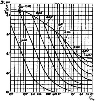
Figure 2.10 Diagram for identification 
2.4 Definition of inshore wave elements
Wave height. Inshore wave height  ,m, shall be defined for specified bottom incline i as per diagrams 2, 3, and 4 (Figure 2.5). Subject to adjustable values
  it can be defined by the diagram
  , as follows .
Wave length. Inshore wave length  ,m, shall be defined as per diagram on Figure 2.9. Subject to adjustable values
  it can be defined using the upper turned curve by the diagram
  , as follows
  .
.
Exceeding of wave over rated level , m, shall be defined using diagram 2.10. Subject to adjustable values  it can be defined using the upper turned curve by the diagram
  , as follows
  .
.
Critical depth Нкр.п. Critical depth subject to the last falling of wave considering constant incline of bottom shall be defined as follows [1]:
 , (2.10)
where  - coefficient as per Table 2.4; n - the number of falling (inclusive of the first one) assumed as n= 2,3,4 as follows
  .
.
For identification of the last falling depth Нкр.п the coefficient kn or the sum of coefficients shall not be assumed less than 0.35. If i>0.005 Нкр.п=Нкр. Surfy area is ended after the critical depth of the last falling.
Table 2.4
Dependence of index from bottom inclines i
| Bottom incline i | 0.01 | 0.015 | 0.02 | 0.025 | 0.03 | 0.035 | 0.04 | 0.045 | 0.05 |
Coefficient 
| 0.75 | 0.63 | 0.56 | 0.5 | 0.45 | 0.42 | 0.4 | 0.37 | 0.35 |
Дата добавления: 2019-02-22; просмотров: 382; Мы поможем в написании вашей работы! |

Мы поможем в написании ваших работ!