Task 3. Heat Transfer Problem (PDE toolbox). Metodology
Task 1. The Wave Equation by Finite Difference Method.
Finite-difference methods are numerical methods for solving differential equations by approximating them with difference equations, in which finite differences approximate the derivatives. FDMs are thus discretization methods.
Similar to the numerical schemes for the heat equation, we can use approximation of derivatives by difference quotients to arrive at a numerical scheme for the wave equation.
The equation of motion is: 
Boundary conditions:
v u(0,t)=0 t ≥ 0
v u(l,t)=0 t ≥ 0
v u(x,0)=f(x) 0 ≤ x ≤ l
clear all; clc;
a=1; %constant
l=1; %boundary for 'x' direction
T=6; %boundary for 't' (time) direction
n=25; %number of steps in 'x' direction
h=l/n; %the length of the step in the 'x' direction
k=h/2; %number of steps in 't' direction
m=T/k; %length of the step in the 't' direction
x(1)=0; %this is determine where will be the start of the coordinates
for i=1:n %we define here the interval of i,
%it can be define in general form as i=1...n,
%also we should remember that MatLab doesn’t allow to start -->
%-->from 0, so we need to start from 1
x(i+1)=x(i)+h; %here we show changes of value by each step in 'x' direction
end
t(1)=0; %this is determine where time will starts if j=1
for j=1:m %we define here the interval of j
t(j+1)=t(j)+k; %we define here the interval of j,
%it can be define in general form as j=1...m -->
%but in this case we need to determine 'm' variable
%which is the step in 't' (time) direction
end
for i=1:n %again we should remember that MatLab doesn’t allow to start -->
%-->from 0, so we need to start from 1
u(i,1)=x(i)*(l-x(i));
u(i,2)=u(i,1)+T*0;
end
for j=1:m;
u(1,j)=0; %This is equal to mu_1
u(l,j)=0; %This is equal to mu_2
end
for j=2:m-1 %don’t put here any ';', because we have here two conditions
i=2:n-1;
u(i,j+1)=2*u(i,j)-u(i,j-1)+(a^2)*(k^2)/(h^2)*(u(i+1,j)-2*u(i,j)+u(i-1,j)); %main formula
end
surf(u); %need to make MatLab plot us a graph

Task 2. The Heat Conduction Equation by Finite Difference Method .
Finite-difference methods are numerical methods for solving differential equations by approximating them with difference equations, in which finite differences approximate the derivatives. FDMs are thus discretization methods.
|
|
|
The heat conduction equation  to determine the temperature u at any point in the bar with length at time t. It is solved in a similar manner to that for the wave equation; the equation differs only in that the right hand side contains a first partial derivative instead of the second.
Boundary conditions:
v u(0,t)=0 t ≥ 0
v u(l,t)=0 t ≥ 0
v u(x,0)=f(x) 0 ≤ x ≤ l
%Solving of the Heat Equation
clear all; clc;
h=0.02; %the step in 'x' direction
l=0.6; %length of interval in the 'x' direction
a=1; %constant
n=l/h; %the number of steps in 'x' direction
m=10; %the number of steps in 't' direction
x(1)=0; %this is determine where will be the start of the coordinates
for i=1:(n+1) %we define here the interval of i,
%it can be define in general form as i=1...n,
%also we should remember that MatLab doesn’t allow to start -->
%-->from 0, so we need to start from 1
x(i+1)=x(i)+h; %here we show changes of value by each step in 'x' direction
end
t(1)=0; %this is determine where time will starts if j=1
T=(h^2)/((a^2)*n); %the step at which time will be evaluated
for j=1:m %we define here the interval of j
t(j+1)=t(j)+T; %we define here the interval of j,
%it can be define in general form as j=1...m -->
%but in this case we need to determine 'm' variable
%which is the step in 't' (time) direction
end
for i=1:(n+1) %don’t put here any ';', because we have here two conditions
j=1:m;
u(i,1)=(3*x(i))*(2-x(i));
u(1,j)=0;
u(n+1,j)=(sqrt(t(j))+2.52);
end
for j=1:m-1 %don’t put here any ';', because we have here two conditions
i=2:n;
u(i,j+1)=u(i,j)+(((a^2)*T)/(h^2))*(u(i+1,j)-2*u(i,j)+u(i-1,j)); %the main formula
end
surf(u); %need to make MatLab plot us a graph

Task 3. Heat Transfer Problem (PDE toolbox). Metodology
|
|
|
This example shows an idealized thermal analysis of a rectangular block with a rectangular cavity in the center. One of the purposes of this example is to show how temperature-dependent thermal conductivity can be modeled in PDE Toolbox.
The partial differential equation for transient conduction heat transfer is:
where T is the temperature, ρ is the material density, Cp is the specific heat, and k is the thermal conductivity. ƒ is the heat generated inside the body which is zero in this example.
Below you can find the Methodology of solving the task by the PDE toolbox application:
1. After opening the PDE toolbox in application folder, we need, firstly, choose a type of solving problem -

2. Then we go the folder “draw” à “rectangle/square”. Draw figure with any dimensions, then another one (smaller) inside first one:

3. Make the double click on the first (R1) figure. After new window appears, we need to put numbers, which define the size and the position of our figure:

For the second figure (R2):

Then we need to change the operator (from ‘+” to “-“) in the command line (“set formula”) above the main workspace to make program cut out figure R2 from figure R1.

After this we need to go to the folder “options” à “axis limits” and put limits for our workspace, as on the following picture.

4. After the third step finish, we can go to the folder “Boundary” à “boundary mode”. Make double click on the leftmost red line (edge). In the window, which will appear, need to set up the temperature to 100 degrees:

Then set up conditions for rightmost edge, where is a heat flux out of the block:

Both top and bottom edges as well as the edges inside the figure are insulated, so there is no heat is transferred across these edges:

5. Now we need to go to the folder “PDE” à “PDE Specification”, where following parameters should be set up:
|
|
|

6. On the next step, we need to generate mesh for our figure. Go to the folder “Mesh” à “Initialize mesh”:
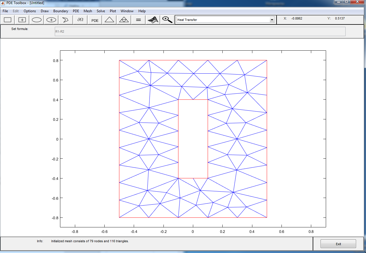
Then choose “Mesh” à “Refine mesh”:

Also need to note, that elements of the mesh should not be larger than 0.2. Go to the folder “Mesh” à “Parameters” and set up 0.2 in the line “Maximum edge size”.

7. After mesh have been set up, we need to go to folder “Solve” à “Parameters”. Choose “Adaptive mode” and leave.

Then again, choose “Solve” à “Solve PDE”. After this, we will get a graph, which MatLab plotted for us.
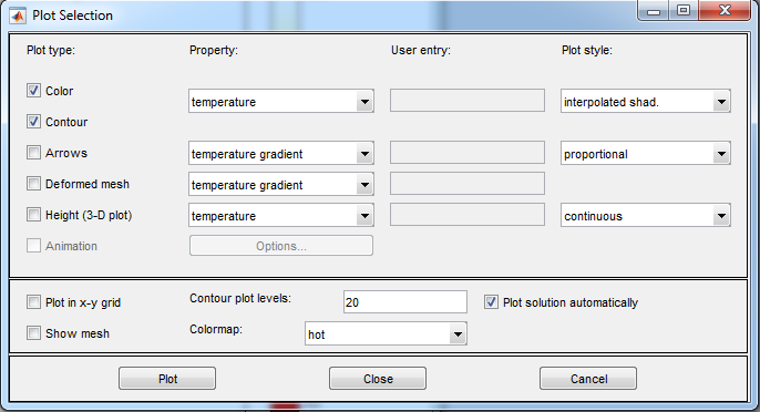
8. The last step is to set up our graph. To do this go to the folder “Plot” à “Parameters”. In window, which will appear, choose “color: temperature”, put mark near the “Contour”, and choose “colormap: hot”. Press the button “Plot”.
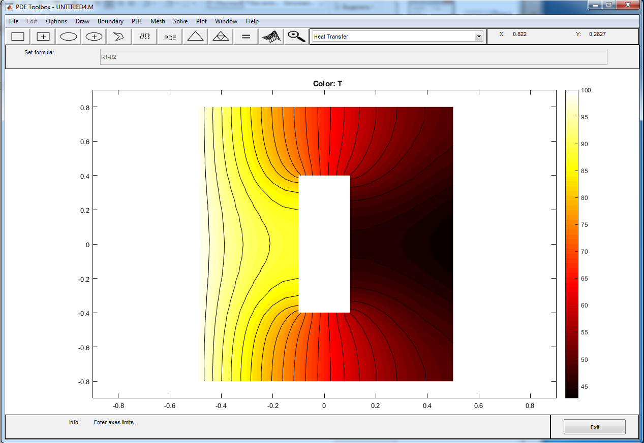
9. Getting the final graph. It should be like following, if everything have been done right:
Дата добавления: 2019-02-22; просмотров: 238; Мы поможем в написании вашей работы! |

Мы поможем в написании ваших работ!