Explicit versus Implicit Costs
Elasticity
Defining and Measuring Elasticity
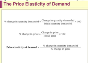
The price elasticity of demand is the ratio of the percent change in the quantity demanded to the percent change in the price as we move along the demand curve (dropping the minus sign).


Using the Midpoint Method
The midpoint method is a technique for calculating the percent change. In this approach, we calculate changes in a variable compared with the average, or midpoint, of the starting and final values.


Interpreting the Price Elasticity of Demand
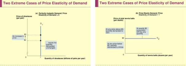
Two Extreme Cases of Price Elasticity of Demand:
Demand is perfectly inelastic when the quantity demanded does not respond at all to changes in the price. When demand is perfectly inelastic, the demand curve is a vertical line.
Demand is perfectly elastic when any price increase will cause the quantity demanded to drop to zero. When demand is perfectly elastic, the demand curve is a horizontal line.
Interpreting the Price Elasticity of Demand
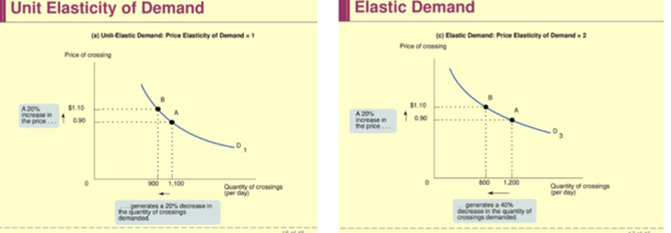
Demand is elastic if the price elasticity of demand is greater than 1.
Demand is inelastic if the price elasticity of demand is less than 1.
Demand is unit-elastic if the price elasticity of demand is exactly 1.
Why Does It Matter Whether Demand is Unit-Elastic, Inelastic, or Elastic?
Because this classification predicts how changes in the price of a good will affect the total revenue earned by producers from the sale of that good.
The total revenue is defined as the total value of sales of a good or service, i.e.
Total Revenue = Price × Quantity Sold

When a seller raises the price of a good, there are two countervailing effects in action (except in the rare case of a good with perfectly elastic or perfectly inelastic demand):
A price effect: After a price increase, each unit sold sells at a higher price, which tends to raise revenue.
A quantity effect: After a price increase, fewer units are sold, which tends to lower revenue.

Elasticity and Total Revenue
If demand for a good is elastic (the price elasticity of demand is greater than 1), an increase in price reduces total revenue. In this case, the quantity effect is stronger than the price effect.
If demand for a good is inelastic (the price elasticity of demand is less than 1), a higher price increases total revenue.In this case, the price effect is stronger than the quantity effect.
If demand for a good is unit-elastic (the price elasticity of demand is 1), an increase in price does not change total revenue.In this case, the sales effect and the price effect exactly offset each other.

Cross-Price Elasticity The cross-price elasticity of demand between two goods measures the effect of the change in one good’s price on the quantity demanded of the other good. It is equal to the percent change in the quantity demanded of one good divided by the percent change in the other good’s price. The Cross-Price Elasticity of Demand between Goods A and B
Cross-Price Elasticity Goods are substitutes when the cross-price elasticity of demand is positive. Goods are complements when the cross-price elasticity of demand is negative.

The Income Elasticity of Demand The income elasticity of demand is the percent change in the quantity of a good demanded when a consumer’s income changes divided by the percent change in the consumer’s income.
Normal Goods and Inferior Goods When the income elasticity of demand is positive, the good is a normal good - that is, the quantity demanded at any given price increases as income increases.When the income elasticity of demand is negative, the good is an inferior good - that is, the quantity demanded at any given price decreases as income increases.

Elasticity of Supply The price elasticity of supply is a measure of the responsiveness of the quantity of a good supplied to the price of that good. It is the ratio of the percent change in the quantity supplied to the percent change in the price as we move along the supply curve.

Two Extreme Cases of Price Elasticity of Supply There is perfectly inelastic supply when the price elasticity of supply is zero, so that changes in the price of the good have no effect on the quantity supplied. A perfectly inelastic supply curve is a vertical line.
There is perfectly elastic supply when even a tiny increase or reduction in the price will lead to very large changes in the quantity supplied, so that the price elasticity of supply is infinite. A perfectly elastic supply curve is a horizontal line. 34
1. Elasticity is a general measure of responsiveness that can be used to answer such questions.
2. The price elasticity of demand—the percent change in the quantity demanded divided by the percent change in the price (dropping the minus sign)—is a measure of the responsiveness of the quantity demanded to changes in the price.
3. The responsiveness of the quantity demanded to price can range from perfectly inelastic demand, where the quantity demanded is unaffected by the price, to perfectly elastic demand, where there is a unique price at which consumers will buy as much or as little as they are offered. When demand is perfectly inelastic, the demand curve is a vertical line; when it is perfectly elastic, the demand curve is a horizontal line.
4. The price elasticity of demand is classified according to whether it is more or less than 1. If it is greater than 1, demand is elastic; if it is less than 1, demand is inelastic; if it is exactly 1, demand is unit-elastic. This classification determines how total revenue, the total value of sales, changes when the price changes.
5. The price elasticity of demand depends on whether there are close substitutes for the good, whether the good is a necessity or a luxury, the share of income spent on the good, and the length of time that has elapsed since the price change.
6. The cross-price elasticity of demand measures the effect of a change in one good’s price on the quantity of another good demanded.
7. The income elasticity of demand is the percent change in the quantity of a good demanded when a consumer’s income changes divided by the percent change in income. If the income elasticity is greater than 1, a good is income elastic; if it is positive and less than 1, the good is income-inelastic.
8. The price elasticity of supply is the percent change in the quantity of a good supplied divided by the percent change in the price. If the quantity supplied does not change at all, we have an instance of perfectly inelastic supply; the supply curve is a vertical line. If the quantity supplied is zero below some price but
infinite above that price, we have an instance of perfectly elastic supply; the supply curve is a horizontal line.
9. The price elasticity of supply depends on the availability of resources to expand production and on time. It is higher when inputs are available at relatively low cost and the longer the time elapsed since the price change.
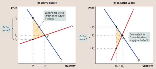
Taxes
Excise tax—a tax charged on each unit of a good or service that is sold.
An excise tax is a tax on sales of a good or service.
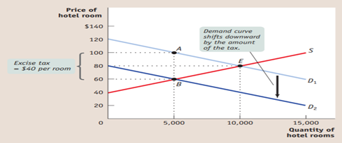


The incidence of a tax is a measure of who really pays it

A tax rate is the amount of tax people are required to pay per unit of whatever is being taxed.

The administrative costs of a tax are the resources used by government to collect the tax, and by taxpayers to pay it, over and above the amount of the tax, as well as to evade it 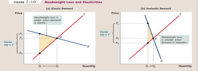
TWO PRINCIPLES OF TAX FAIRNESS
Fairness, like beauty, is often in the eyes of the beholder. When it comes to taxes, however, most debates about fairness rely on one of two principles of tax fairness: the benefits principle and the ability-to-pay principle.
According to the benefits principle of tax fairness, those who benefit from public spending should bear the burden of the tax that pays for that spending. For example, those who benefit from a road should pay for that road’s upkeep, those who fly on airplanes should pay for air traffic control, and so on.
The benefits principle is attractive from an economic point of view because it matches well with one of the major justifications for public spending—the theory of public goods, which will be covered in Chapter 18.
According to the benefits principle of tax fairness, those who benefit from public spending should bear the burden of the tax that pays for that spending.
According to the ability-to-pay principle of tax fairness, those with greater ability to pay a tax should pay more tax.
A lump-sum tax is the same for everyone, regardless of any actions people take
In a well-designed tax system, there is a trade-off between equity and efficiency: the system can be made more efficient only by making it less fair, and vice versa


International Trade
Goods and services purchased from abroad are imports; goods and services sold abroad are exports.
Globalization is the phenomenon of growing economic linkages among countries.
opportunity cost on the example of shrimp
To produce shrimp, any country must use resources-land, labour, capital, and so on-
that could be used to produce other things. The potential production of other
goods that a country must give up in order to produce a ton of shrimp is the opportunity cost of that
ton. So, the opportunity cost of a ton of shrimp, in terms of other goods such as
computers, is much less in Vietnam than it is in the United States.
And we can say that Vietnam has a comparative advantage in producing shrimp.
Comparative Advantage
People can get a lot more products and services if they share, for example, the US and Vietnam should produce their computers, but without the trade such as the United States will produce 1000 computers and 500 shrimp and international trade the United States will produce 2000 computers that are reserved for a 1250, and the remaining 750 will give Vietnam that will go well, and at the end instead of 1000 computers in the USA will be 1250 instead of 500 shrimp they will be 750
The Ricardian model of international trade analyzes international trade under the assumption that opportunity costs are constant.
Autarky is a situation in which a country does not trade with other countries.


The factor intensity of production of a good is a measure of which factor is used in relatively greater quantities than other factors in production.
The main sources of comparative advantage are international differences in climate, factor endowments, and technology.
According to the Heckscher–Ohlin model, a country has a comparative advantage in a good whose production is intensive in the factors that are abundantly available in that country.
For example, oil refineries use much more capital per worker than garment factories. So, according to the theory, a country with a relative abundance of capital will have a comparative advantage in capital-intensive industries, such as oil refining, but a country with a relative abundance of labor will have a comparative advantage in labor-intensive industries, such as clothing manufacturing.
The domestic demand curve shows how the quantity of a good demanded by domestic consumers depends on the price of that good.
The domestic supply curve shows how the quantity of a good supplied by domestic producers depend on the price of that good.
Consumer and Producer Surplus in Autarky
The domestic demand curve reflects only the demand of residents of our own country. Similarly, the domestic supply curve shows how the quantity of a good supplied by producers inside our own country depends on the price of that good.

the country opens the import market. It can buy unlimited quantities of shrimp, for example, shrimp will cost at the world price of Pw, if this price is less than the domestic one, we can conclude that it is more profitable to import.

Tariff
A tariff is a form of excise tax, one that is levied only on sales of imported goods.

before the tariff was introduced, the price dropped to PW QD-QS were at these points. But then, after the introduction of the tariff, imports become unprofitable, if the domestic price is not equal to the world price plus the tariff, then the domestic price will rise to pt Domestic production rises to QST, domestic consumption falls to QDT, and imports fall to QDT – QST.
MAKING DECISION
opportunity cost—that is, the real cost of something is what you must give up to get it. When making decisions, it is crucial to think in terms of opportunity cost, because the opportunity cost of an action is often considerably more than the cost of any outlays of money. All costs are opportunity costs. They can be divided into explicit costs and implicit costs.
Explicit versus Implicit Costs
Explicit costs are out-of-pocket costs, that is, payments that are actually made. Wages that a firm pays its employees or rent that a firm pays for its office are explicit costs.
An implicit cost does not require an outlay of money; it is measured by the value, in dollar terms, of benefits that are forgone. For example, time of training new employees
Many cost have both implicit cost and explicit cost. For example, if a machine in a factory breaks down, the money to repair the machine is explicit cost, the revenue lost during the repair is an implicit cost
Economic cost is the sum of implicit cost and explicit cost. For example, a person decided to wait for an hour to buy a phone and didn’t go to work. The exp cost of the phone is $200, the imp cost of the work hour is $30. The economic cost is $230.
Дата добавления: 2022-06-11; просмотров: 35; Мы поможем в написании вашей работы! |

Мы поможем в написании ваших работ!